Stratum Retention Policies

The following compares procedures for stratum pruning in hereditary stratigraphy. Read here for a general introduction to the stratum deposition process.

Note that here we use “algorithm” to connote general classes of stratum retention strategies and “policy” to connote a specific strategy within an algorithmic class. Put another way, a policy is a parametrized algorithm.

Visualizing Policy Behavior

No History	Retained History	All History

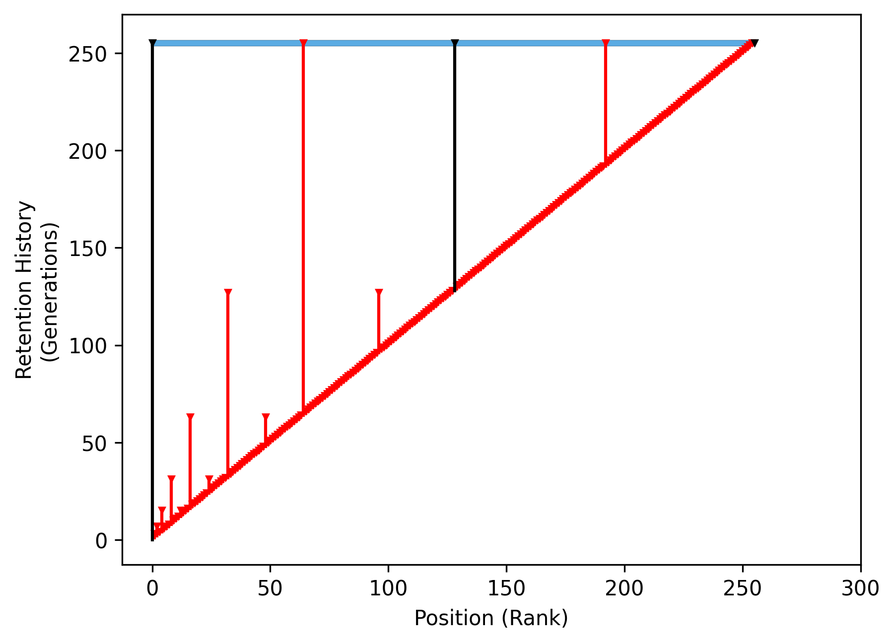
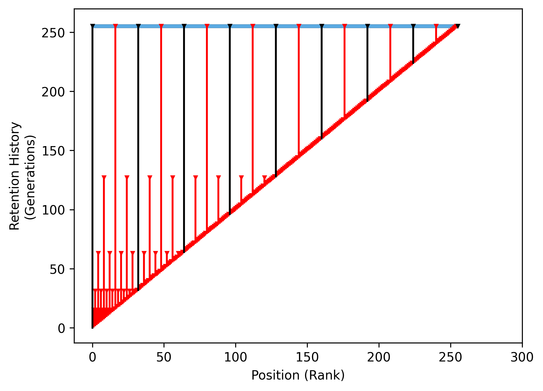
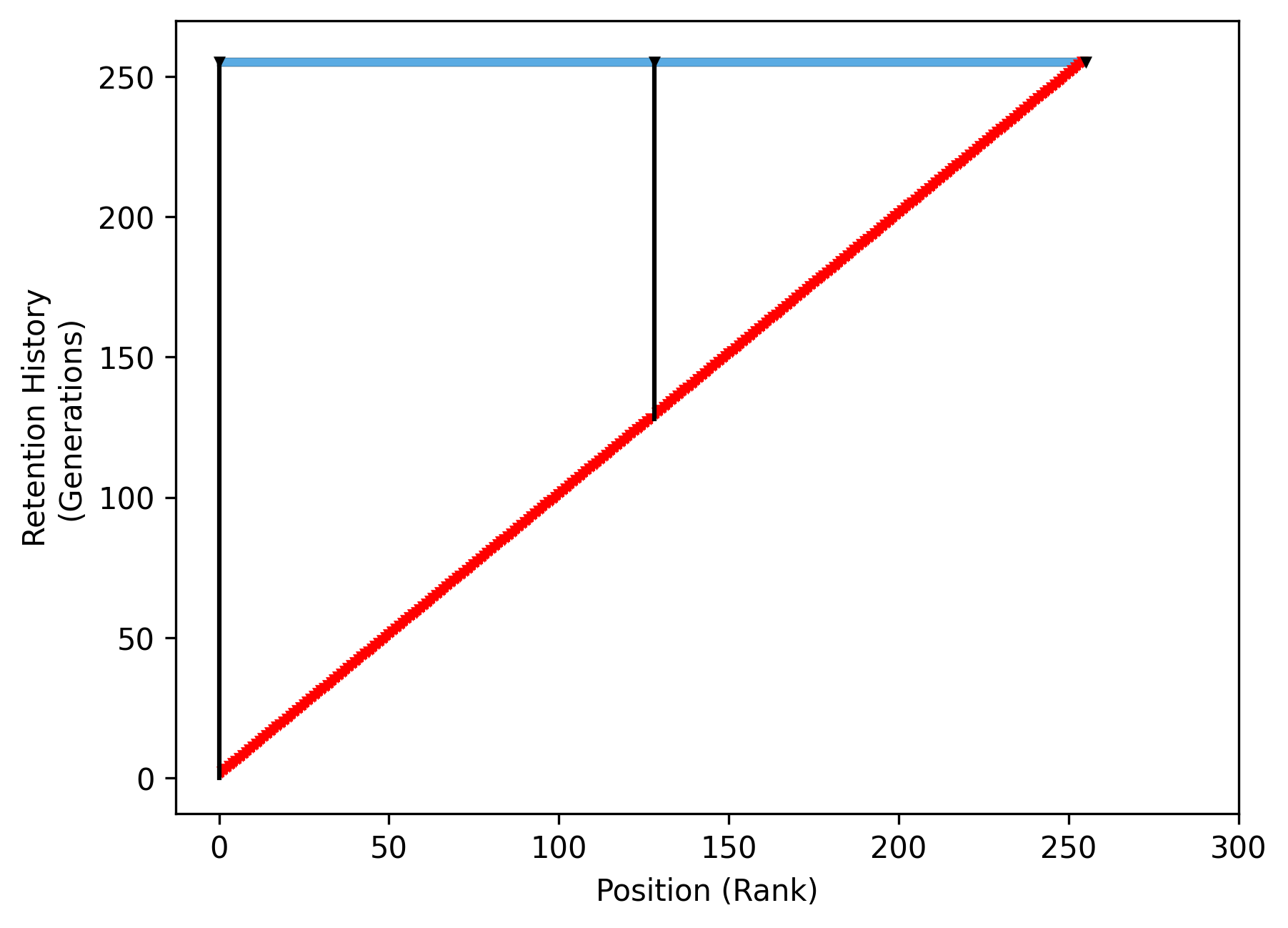
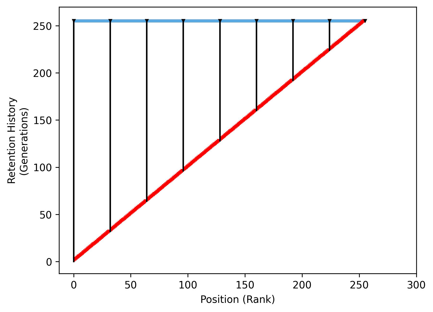
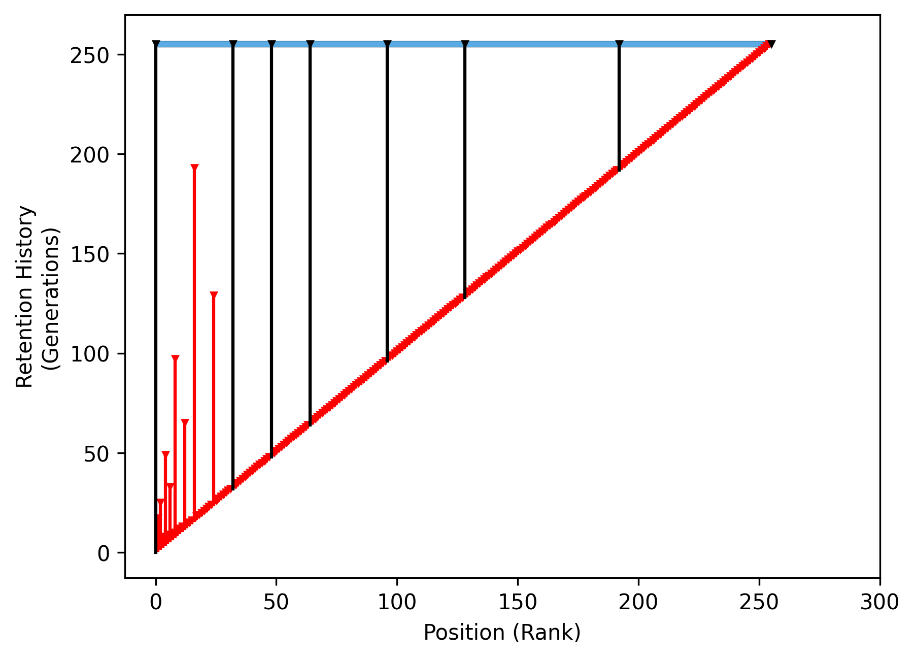
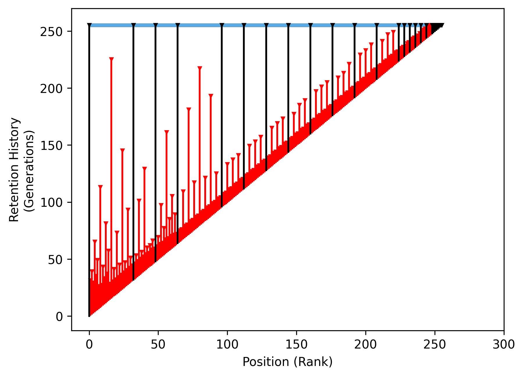
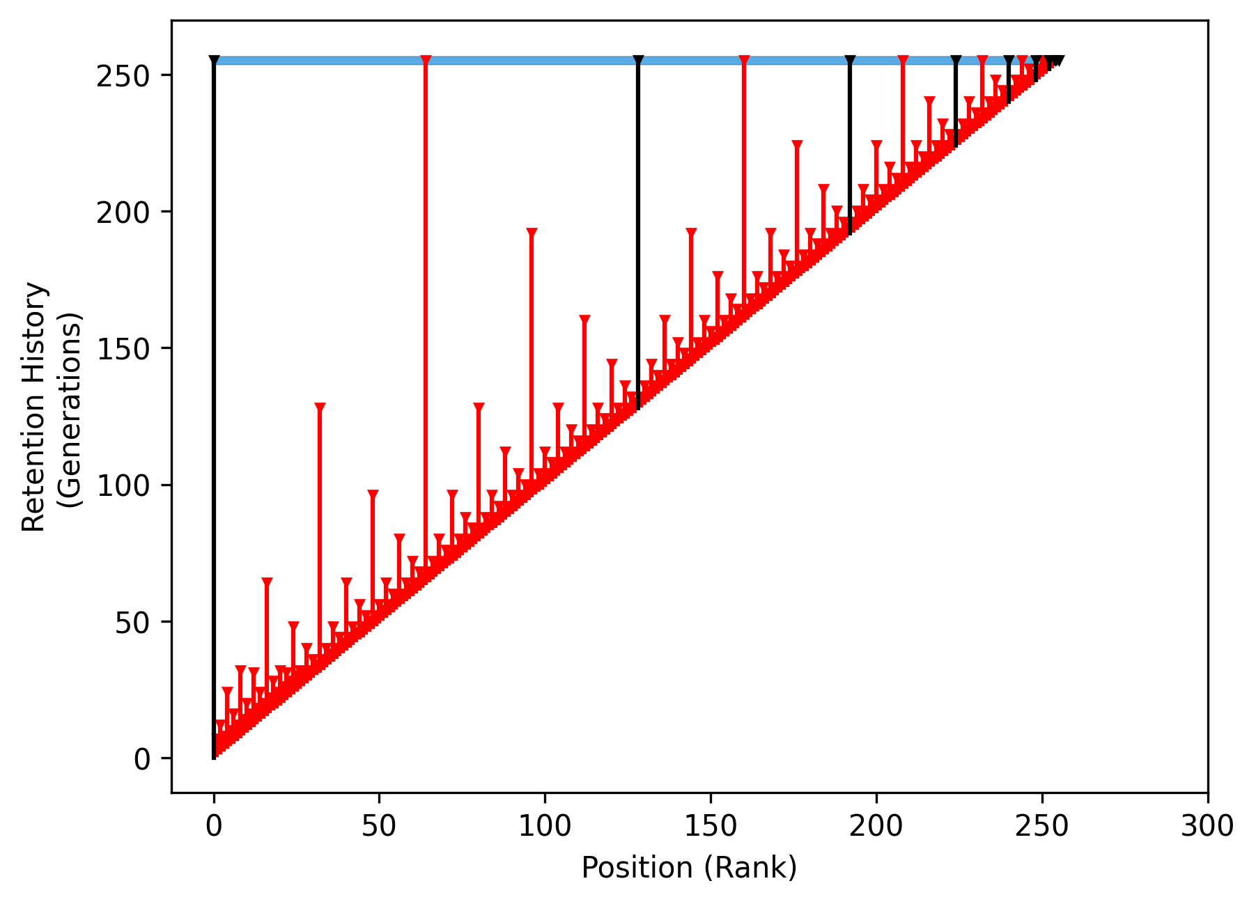
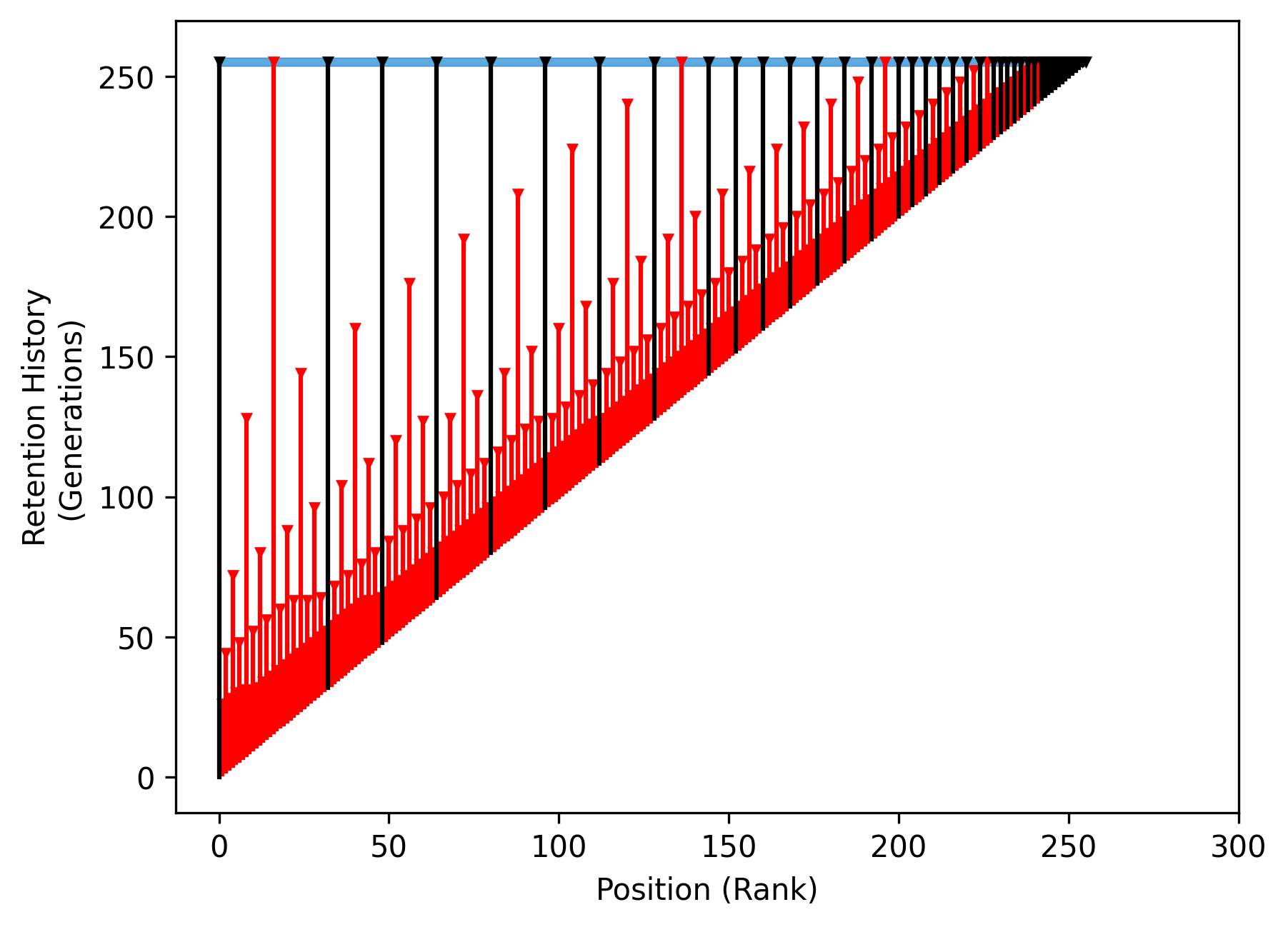
Because stratum retention policies unfold across space and time (i.e., the location of pruned strata and the generations at which they are pruned), the retention drip plot visualizations we use to depict them require a bit of explanation to get up to speed with. This section builds up the visualizations step-by-step in the table above. (Note that the animations loop at 256 generations; if you are impatient you can refresh the page to restart the animations.)

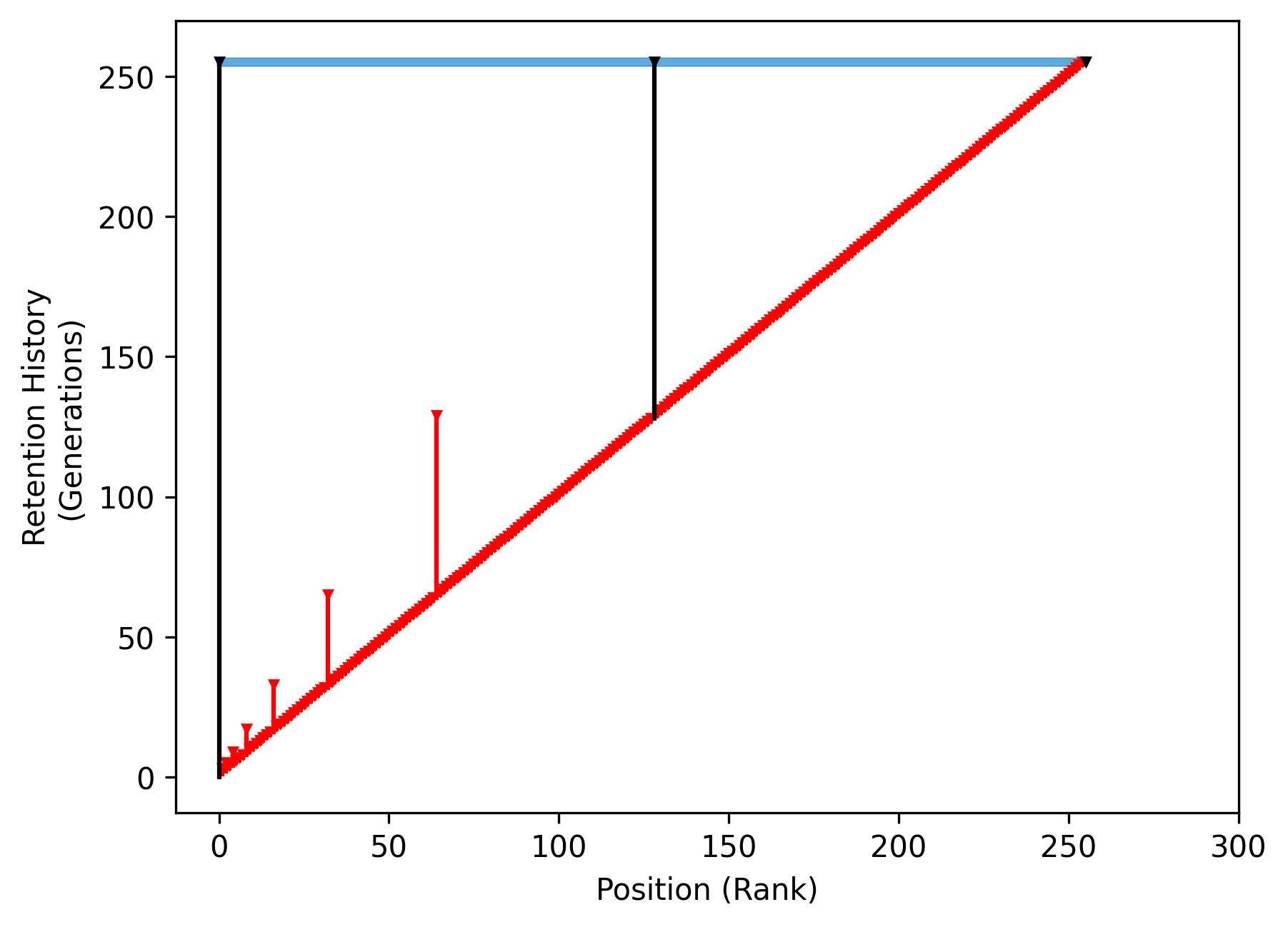
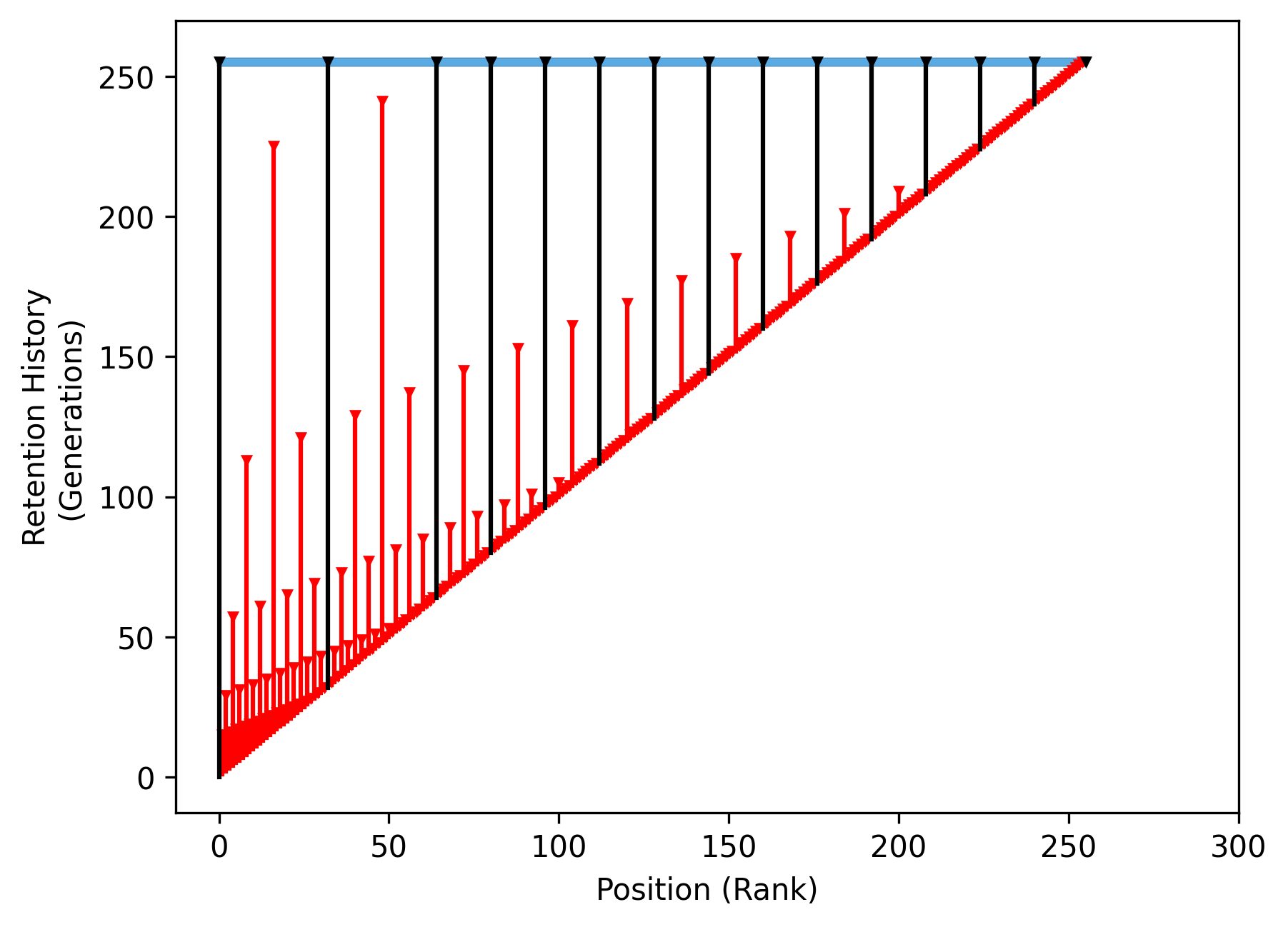
The leftmost column animates the evolution of a single hereditary stratigraphic column over generations with no historical overlay. The column itself is shown “tipped over,” appearing as a horizontal blue rectangle. Upside-down triangles are stratum within the column. The position of strata in the x dimension correspond to the generation of their deposition; new strata are appended on the right. Retention status is depicted with color. Black strata are retained and red strata have been pruned.

The center column uses the y dimension to introduce historical traces for retained strata. The line below each retained stratum spans from the generation it was deposited to the current generation. Note that the column itself is positioned at the current generation at the top of the diagram.

Finally, the rightmost column further layers on historical traces of pruned strata. Instead of having their trace deleted when pruned, their trace is turned red and frozen in place. So, red traces span from the generation a pruned stratum was deposited to the generation it was pruned.

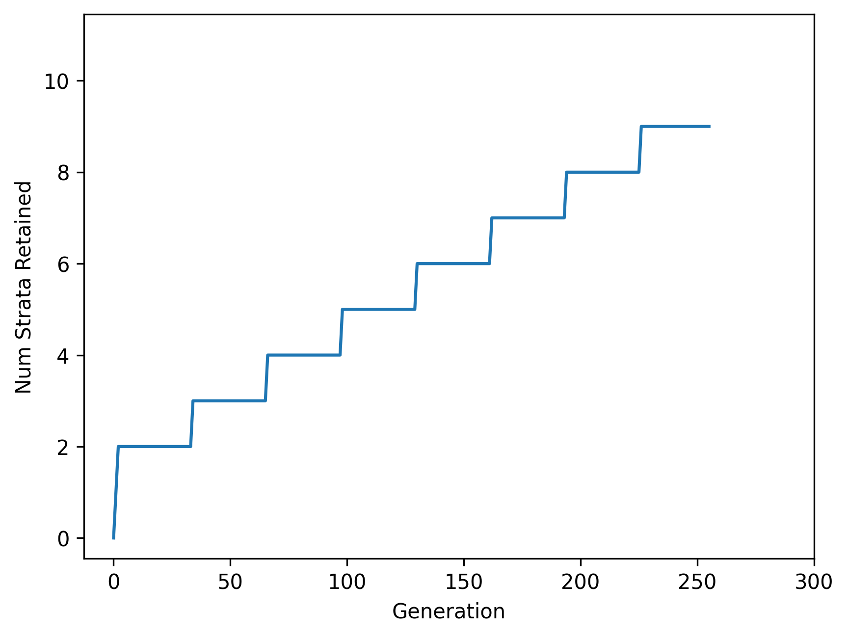
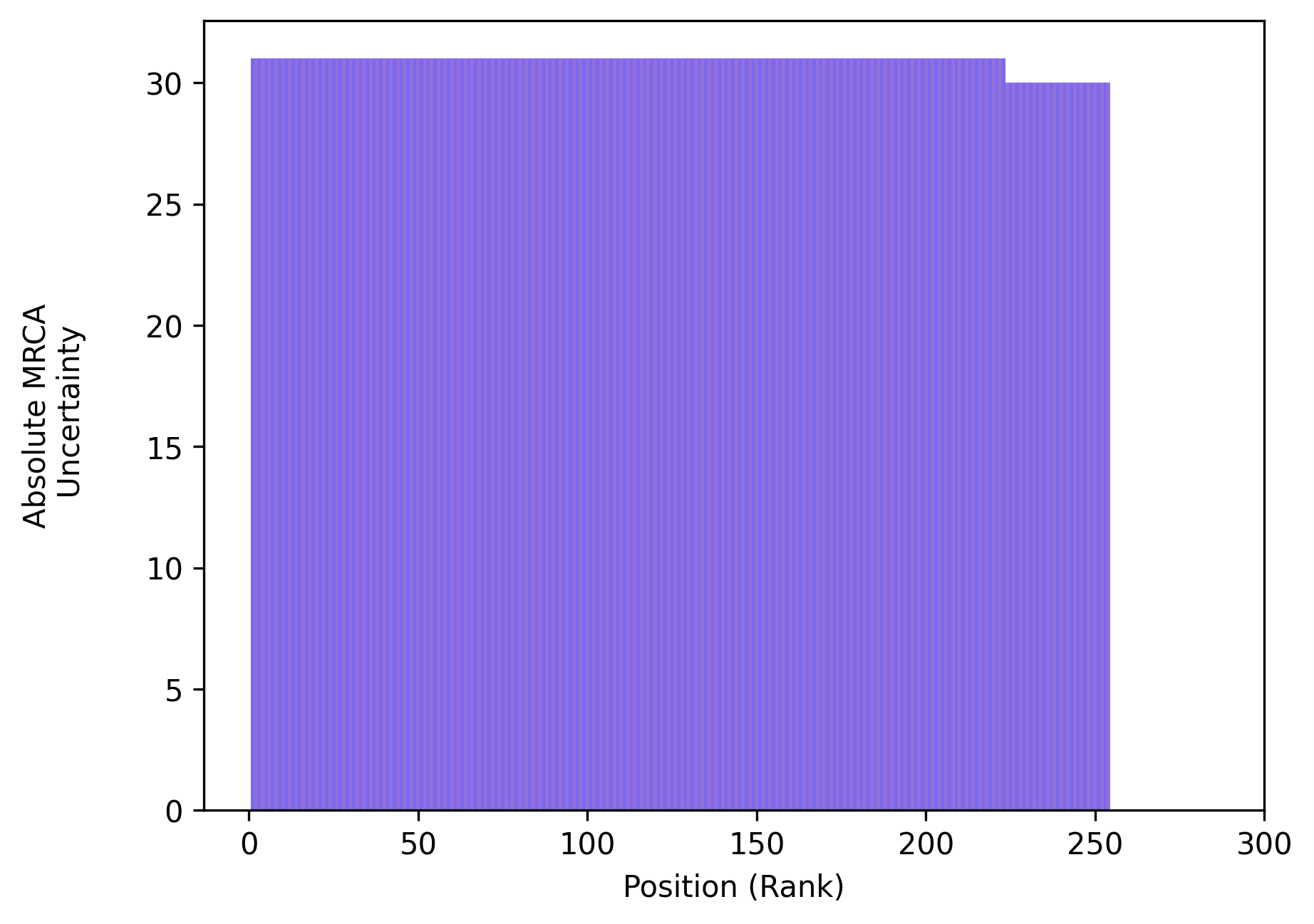
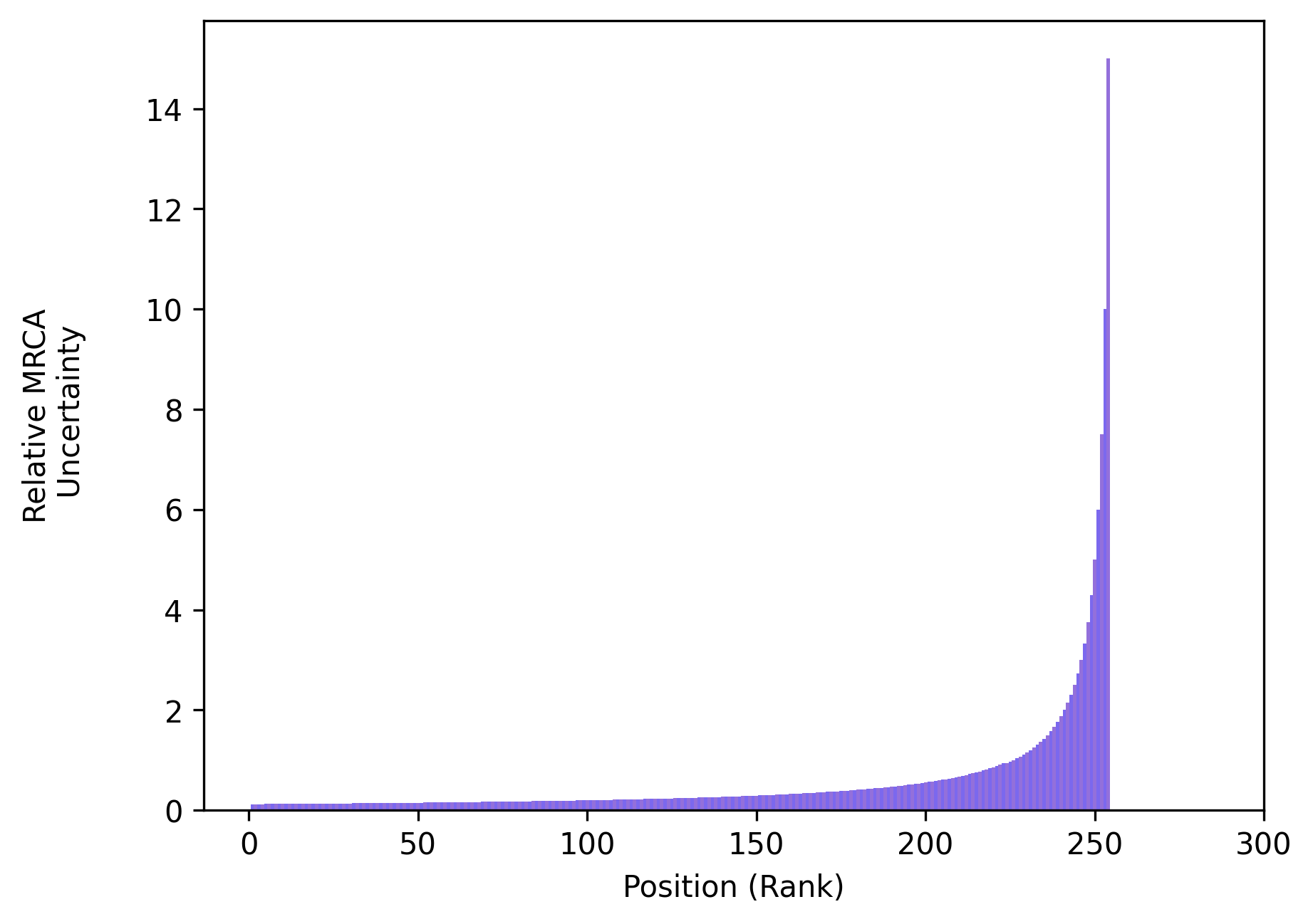
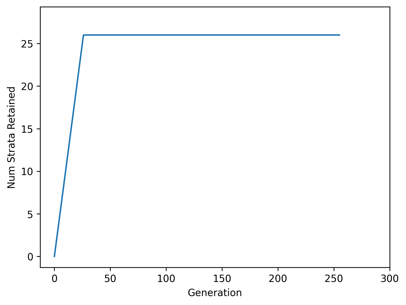
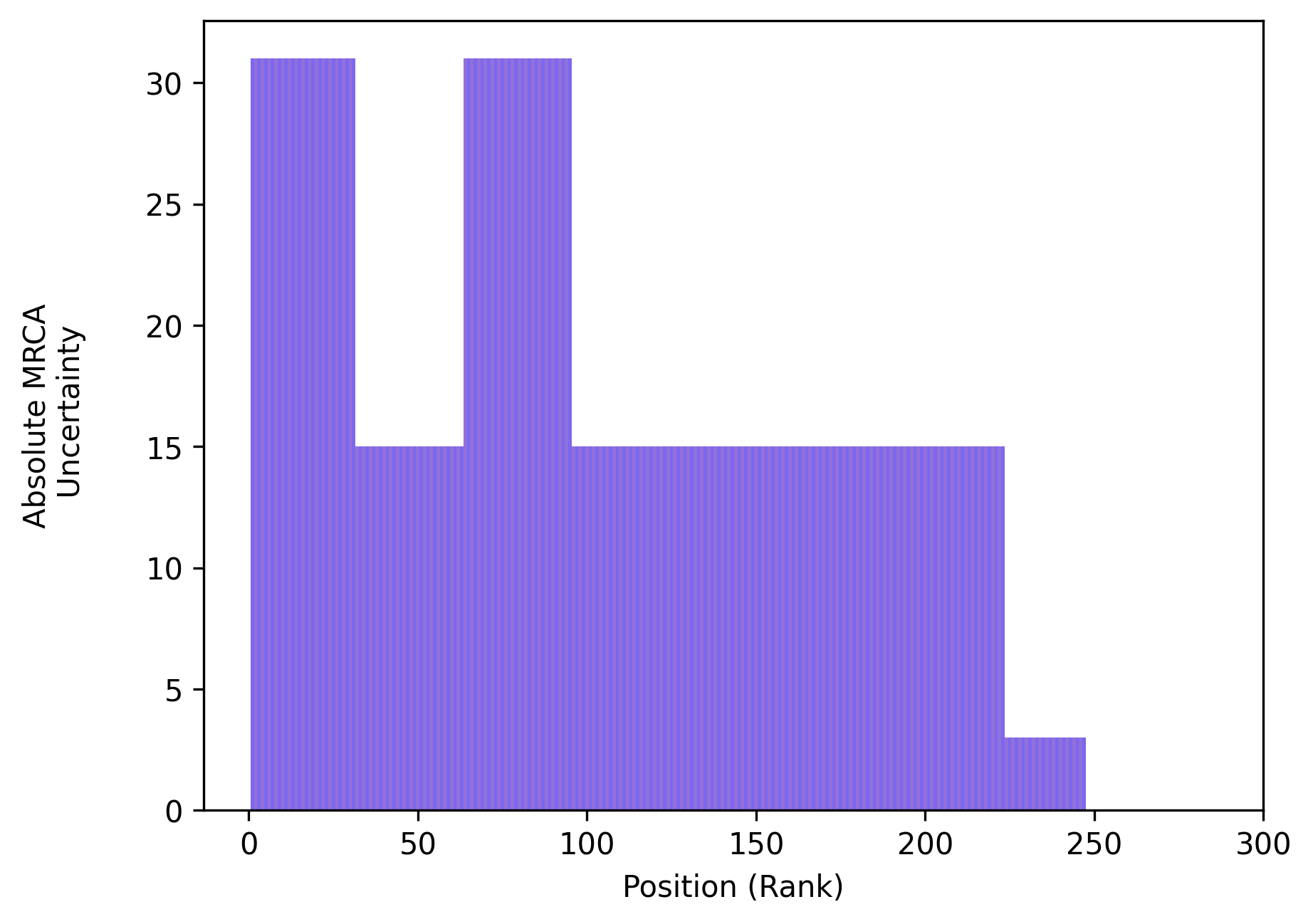
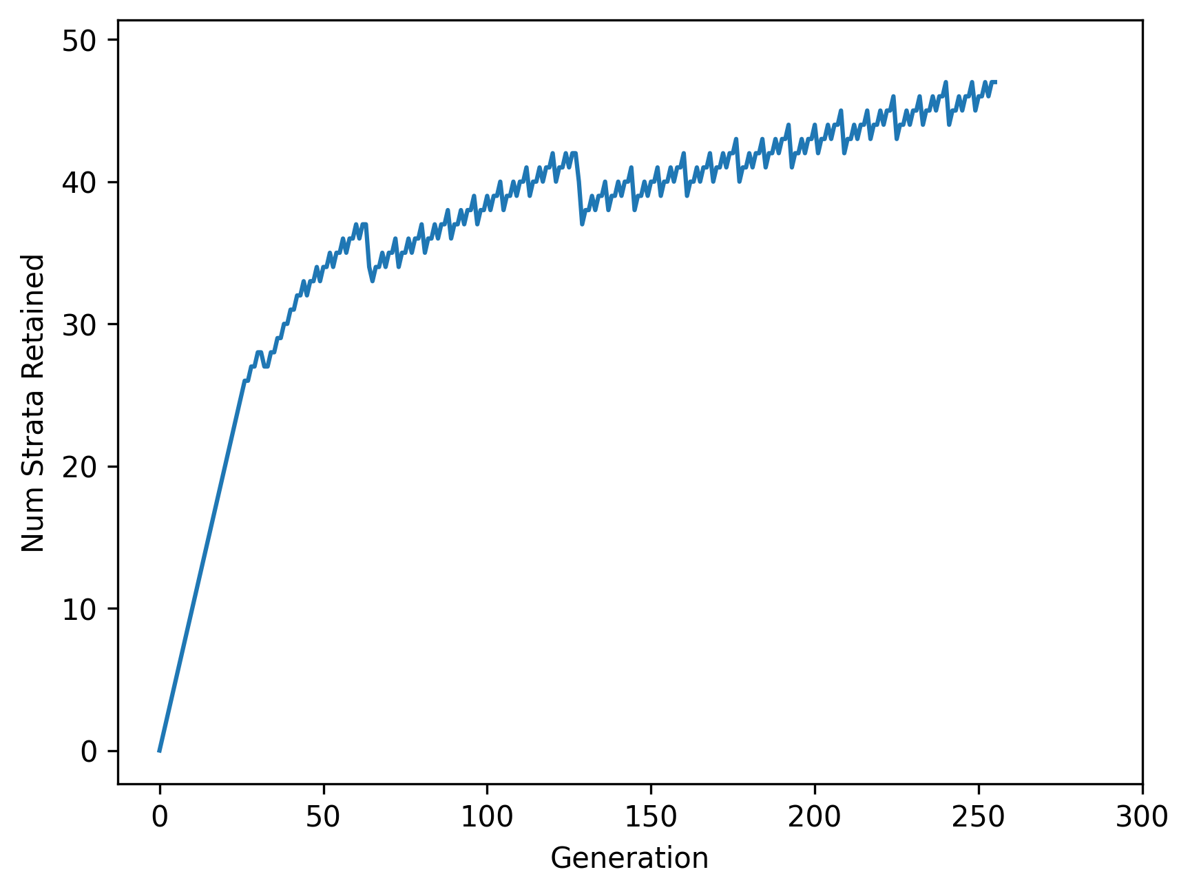
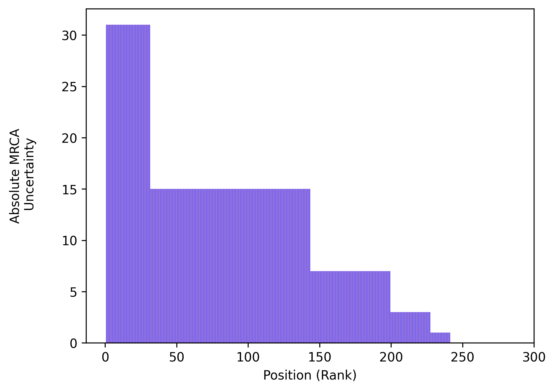
Animated panels below situate this visualization alongside additional graphs depicting absolute and relative estimation error across possible MRCA generations as well as relative and absolute column size (i.e., number of strata retained). Two policy instantiations are visualized for each algorithm — one yielded from a sparse parameterization and the other from a dense parameterization (i.e., one configured to retain fewer strata and one configured to retain more).

Choosing a Retention Algorithm

The space-vs-resolution and distribution-of-resolution trade-offs of library-provided stratum retention algorithms are summarized below.

Stratum Retention Algorithm	Space Complexity	MRCA Gen Uncertainty
Fixed Resolution Algorithm	`n/k`	`k`
Recency-proportional Resolution Algorithm	`k * log(n)`	`m/k`
Depth-proportional Resolution Algorithm	`k`	`n/k`
Geometric Sequence Nth Root Algorithm	`k`	`m * n^(1/k)`
Curbed Recency-proportional Resolution Algorithm	`k`	`m / k` -> `m * n^(1/k)`

where n is generations elapsed, m is generations since MRCA, and k is an arbitrary user-determined constant.

Note that distribution-of-resolution trade-offs are described via the definition of uncertainty bounds in terms of generations since MRCA m versus overall generations elapsed n.

The hstrat library includes a suite of variants for several of these stratum retention algorithms. These variants differ in terms of secondary considerations, for example whether column size exactly traces the asymptotic guarantee or fluctuates around it. Computational intensity to calculate the set of strata to be dropped at each generation may also differ between variants.

The next sections tour available stratum retention algorithms in detail.

Parameterizing a Retention Policy

Stratum retention algorithms can be automatically parameterized for desired properties. For example, you may want to produce a policy from a particular algorithm that retains at most 100 strata at generation 1 million.

Two components are required to perform a parameterization.

The first, an “evaluator” controls which policy property is being parameterized for. Available options are

MrcaUncertaintyAbsExactEvaluator
MrcaUncertaintyAbsUpperBoundEvaluator
MrcaUncertaintyRelExactEvaluator
MrcaUncertaintyRelUpperBoundEvaluator
NumStrataRetainedExactEvaluator
NumStrataRetainedUpperBoundEvaluator

The second, a “parameterizer” controls whether the policy property should be paramaterized to be greater than, equal, or less than equal a target value. Available options are

PropertyAtMostParameterizer
PropertyAtLeastParameterizer
PropertyExactlyParameterizer

The evaluator should be provided as an argument to parameterizer, which should in turn be provided as an argument to the algorithm’s Policy initializer.

stratum_retention_policy = hstrat.geom_seq_nth_root_tapered_algo.Policy(
    parameterizer=hstrat.PropertyAtMostParameterizer(
        target_value=127,
        policy_evaluator \
            =hstrat.MrcaUncertaintyAbsExactEvaluator(
                at_num_strata_deposited=256,
                at_rank=0,
        ),
    ),
)

Depth Proportional Resolution Algorithm

The depth proportional resolution algorithm drops half of retained strata when a threshold size cap is met in order to maintain O(1) space complexity. Retained strata are evenly spaced.

Sparse Parameterization	Dense Parameterization

Dense Parameterization Detail

Num Strata Retained	Absolute MRCA Uncertainty by Position	Relative MRCA Uncertainty by Position

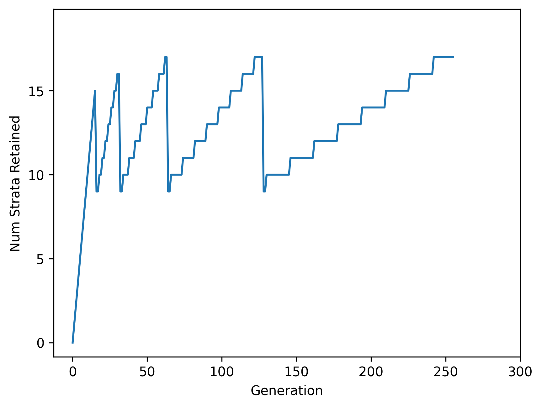
Tapered Depth Proportional Resolution Algorithm

The tapered depth proportional resolution algorithm drops strata gradually from the rear once the threshold size cap is met (instead of purging half of strata all at once).

Sparse Parameterization	Dense Parameterization

Dense Parameterization Detail

Num Strata Retained	Absolute MRCA Uncertainty by Position	Relative MRCA Uncertainty by Position

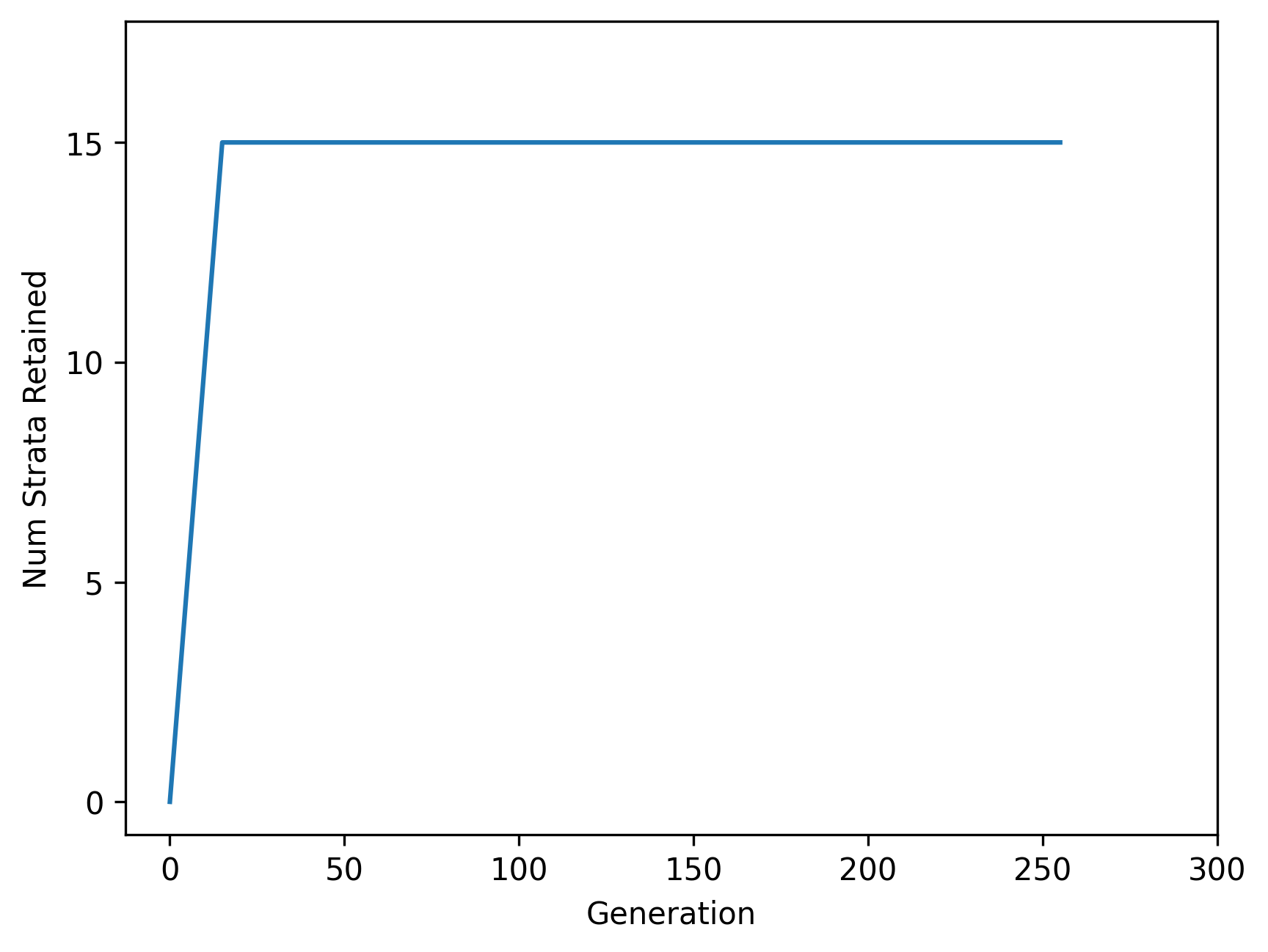
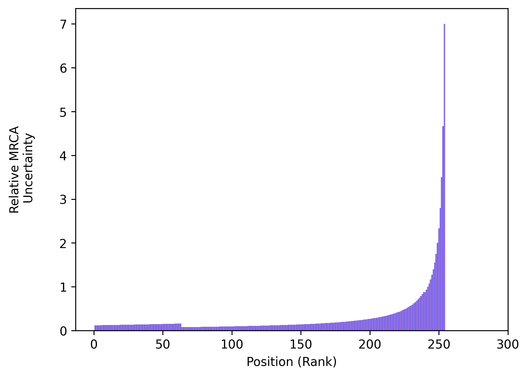
Fixed Resolution Algorithm

The fixed resolution algorithm permanently retains every nth stratum, giving it linear O(n) space complexity and uniform distribution of retained strata.

Sparse Parameterization	Dense Parameterization

Dense Parameterization Detail

Num Strata Retained	Absolute MRCA Uncertainty by Position	Relative MRCA Uncertainty by Position

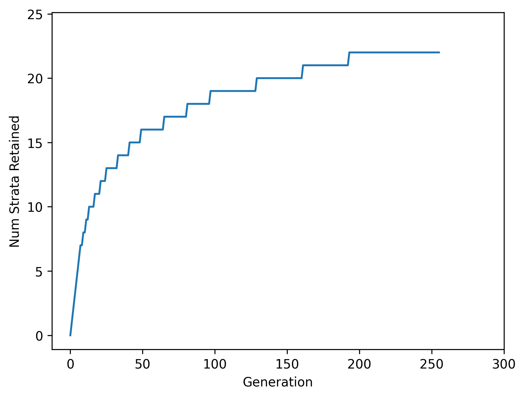
Geometric Sequence Nth Root Algorithm

The geometric sequence algorithm provides constant O(1) space complexity with recency-proportional distribution of retained strata. To accomplish this, a fixed number k of fixed-cardinality subcomponents track k waypoints exponentially spaced backward from the most-recent stratum (i.e., spaced corresponding to the roots 0/k, 1/k, 2/k, …, k/k).

Sparse Parameterization	Dense Parameterization

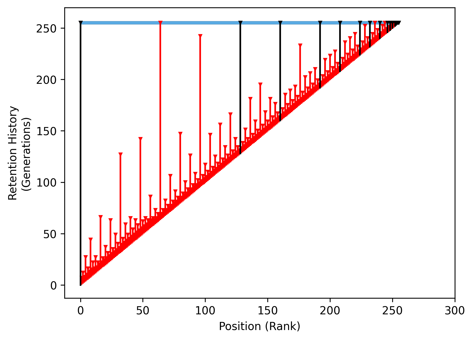
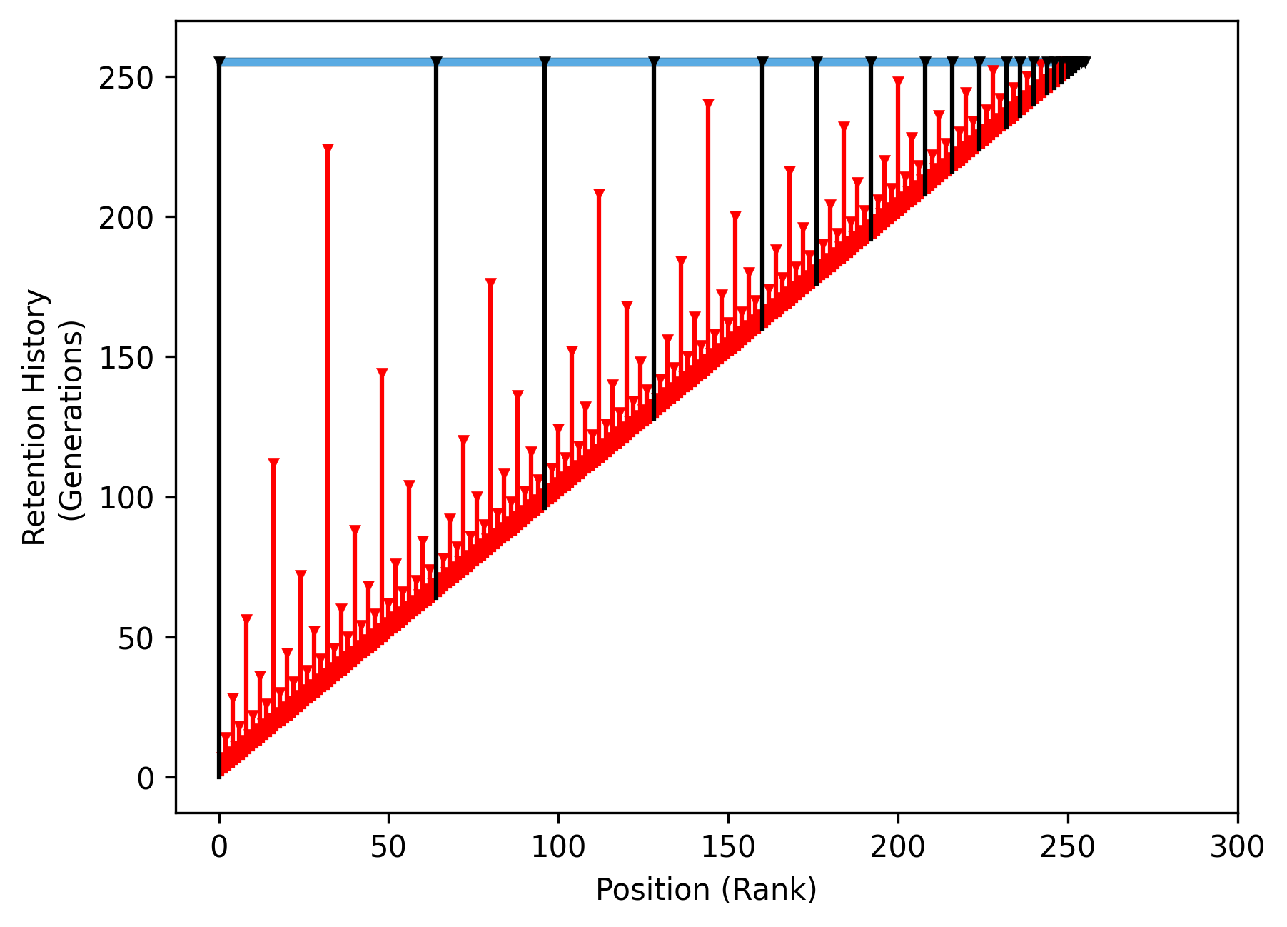
Dense Parameterization Detail

Num Strata Retained	Absolute MRCA Uncertainty by Position	Relative MRCA Uncertainty by Position

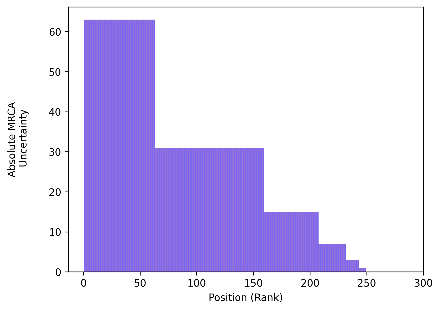
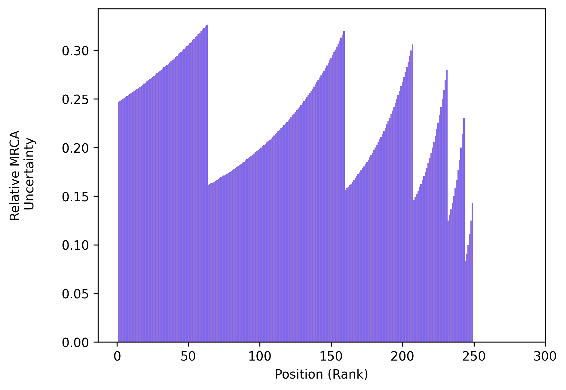
Tapered Geometric Sequence Nth Root Algorithm

The tapered geometric sequence nth root algorithm maintains exactly-constant size at its vanilla counterpart’s upper bound instead of fluctuating below that bound. It is more computationally expensive than the vanilla geometric sequence nth root algorithm.

Sparse Parameterization	Dense Parameterization

Dense Parameterization Detail

Num Strata Retained	Absolute MRCA Uncertainty by Position	Relative MRCA Uncertainty by Position

Recency Proportional Resolution Algorithm

The recency proportional resolution algorithm maintains relative MRCA estimation error below a constant bound. It exhibits logarithmic O(log(n)) space complexity.

Sparse Parameterization	Dense Parameterization

Dense Parameterization Detail

Num Strata Retained	Absolute MRCA Uncertainty by Position	Relative MRCA Uncertainty by Position

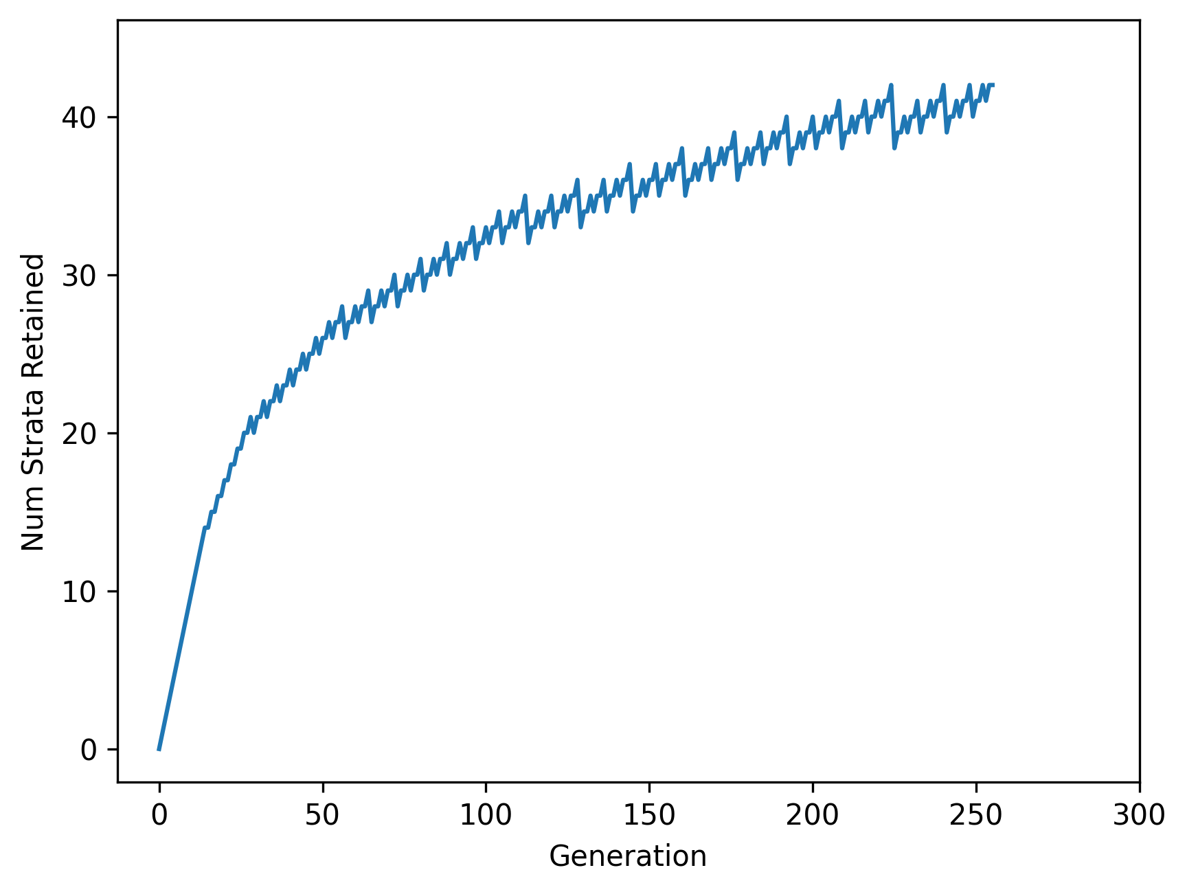
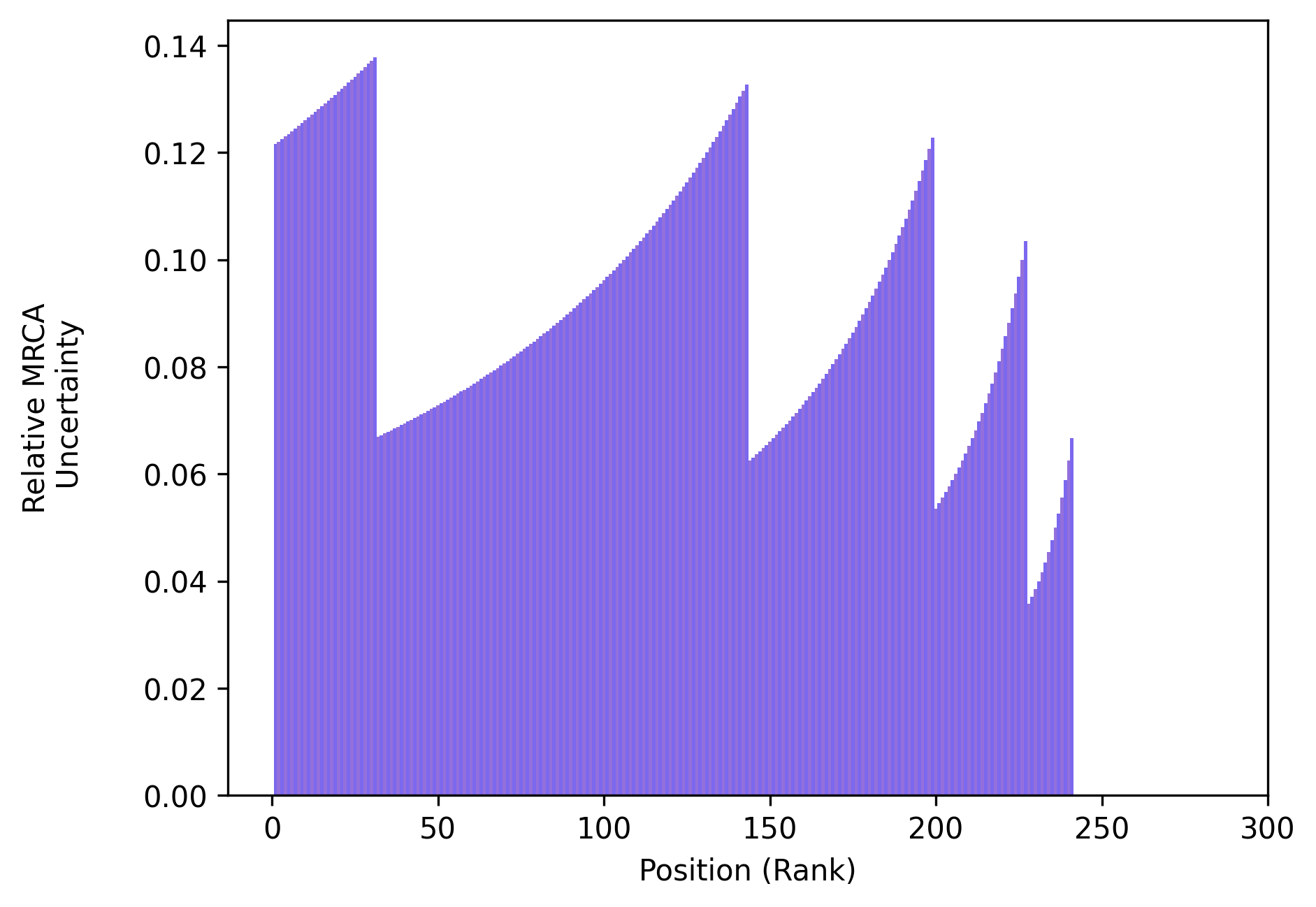
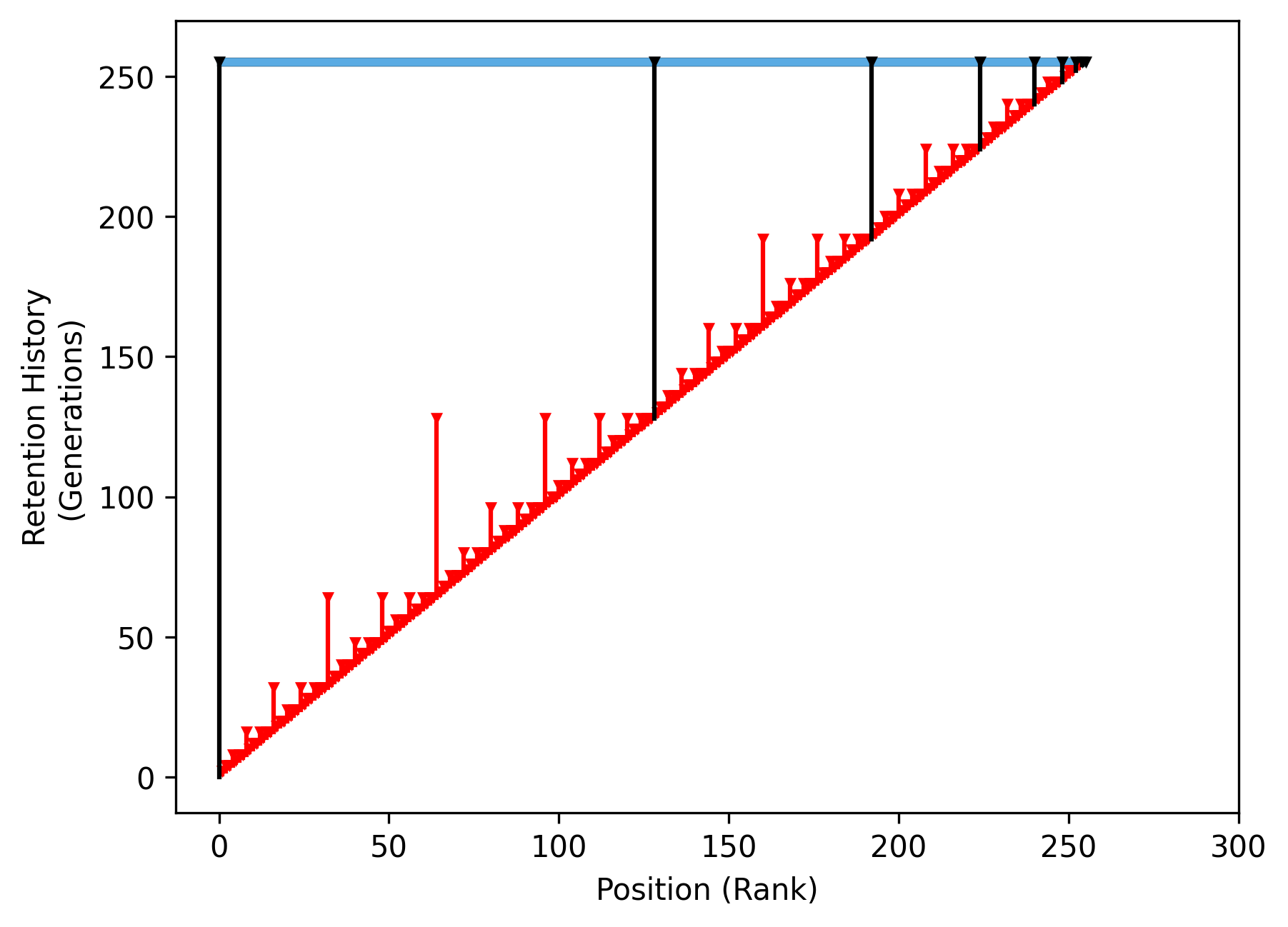
Curbed Recency Proportional Resolution Algorithm

The curbed recency-proportional resolution algorithm eagerly utilize fixed stratum storage capacity to minimize recency-proportional MRCA uncertainty.

This strategy provides the finest-possible recency-proportional granularity within parameterized space constraint. Resolution degrades gracefully as deposition history grows.

This algorithm is similar to the geometric sequence nth root algorithm in guaranteeing constant space complexity with recency-proportional MRCA uncertainty. However, this curbed recency-proportional algorithm makes fuller (i.e., more aggressive) use of available space during early depositions.

In this way, it is similar to the tapered geometric sequence nth root algorithm during early depositions. The tapered nth root algorithm makes fullest use of fixed available space. In fact, it perfectly fills available space. However, the curbed recency-proportional algorithm’s space use is more effective at early time points — it better minimizes recency-proportional MRCA uncertainty than the curbed algorithm.

Sparse Parameterization	Dense Parameterization

Dense Parameterization Detail

Num Strata Retained	Absolute MRCA Uncertainty by Position	Relative MRCA Uncertainty by Position

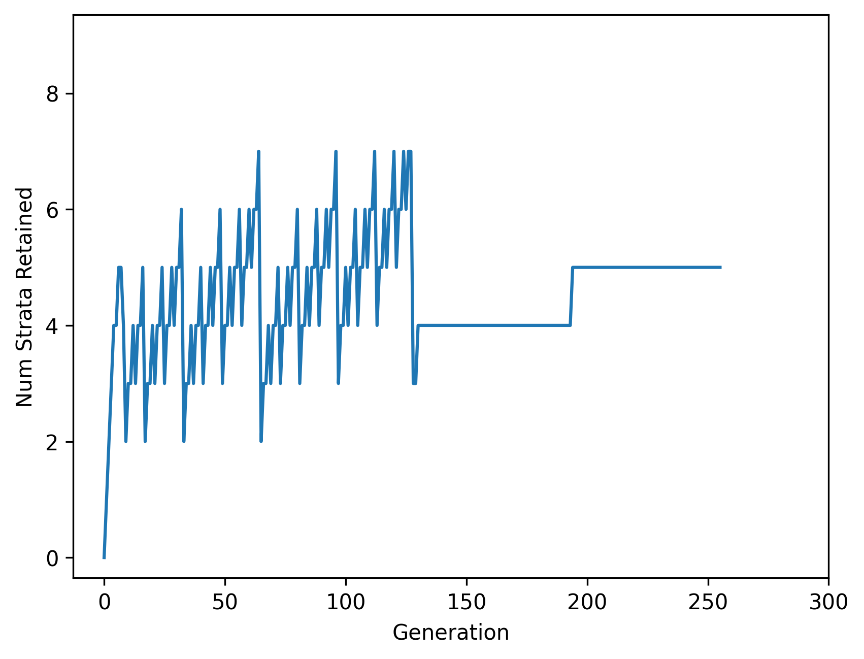
This policy works by splicing together successively-sparser recency_proportional_resolution_algo paramaterizations then a permanently fixed parameterization of the geometric_seq_nth root algorithm. Sparsification occurs when upper bound space use increases to exceed the fixed-size available capacity. For a very sparse paramaterization with a size cap of eight strata, shown below, the transition to geometric_seq_nth_root_ago can be seen at generation 129.

Very Sparse Parameterization

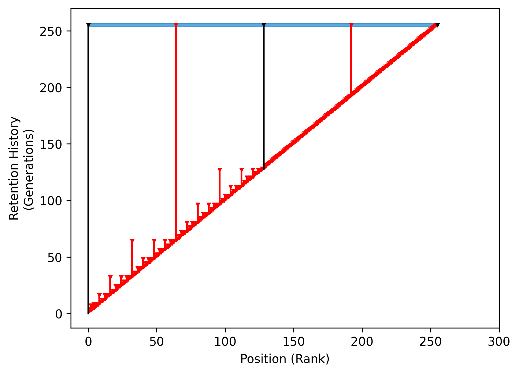
Note: minor changes have been made to the transition points of the curbed-recency proportional resolution algorithm, but these older graphics best convey the underlying concept behind the algorithm.

Very Sparse Parameterization Detail

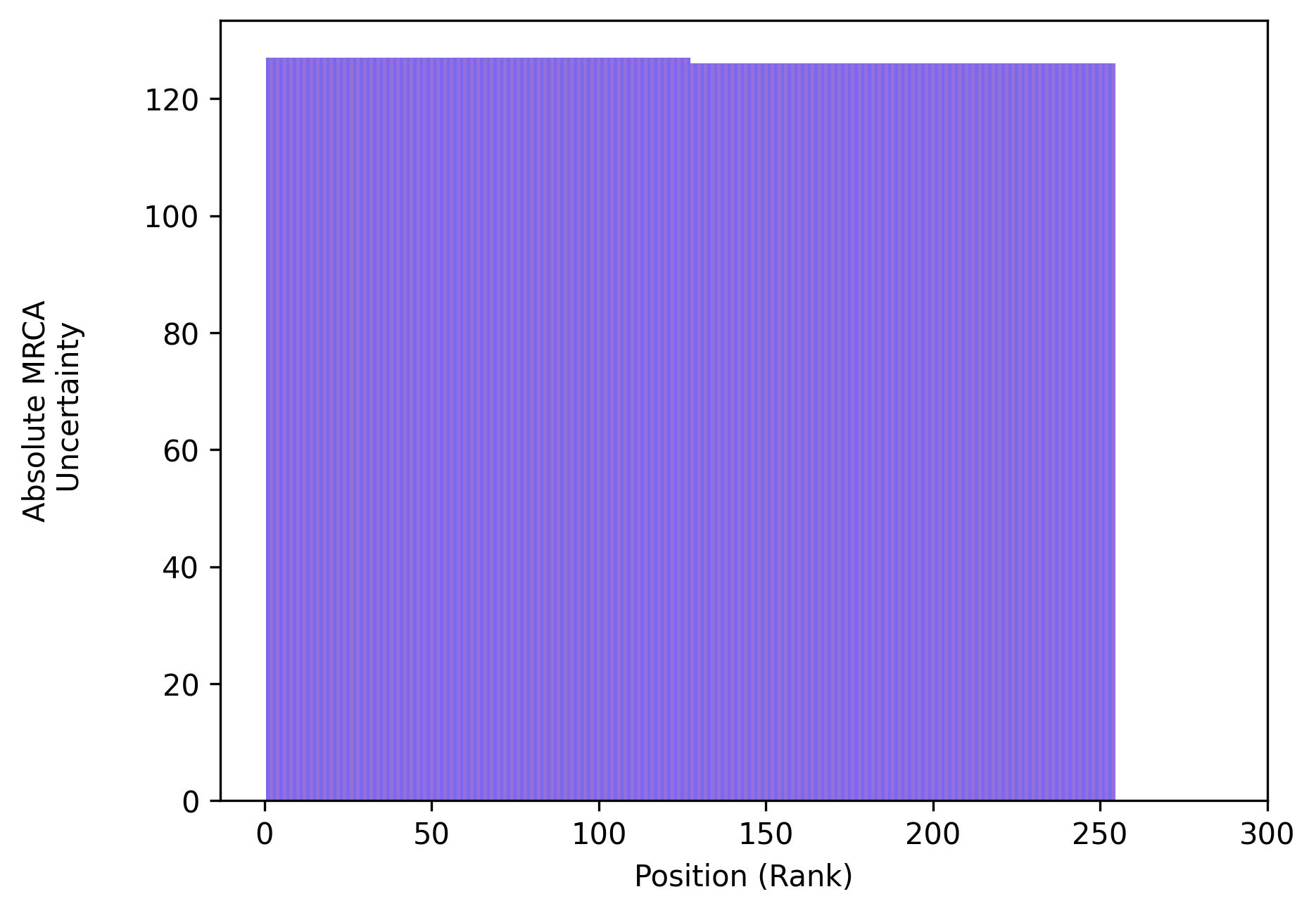
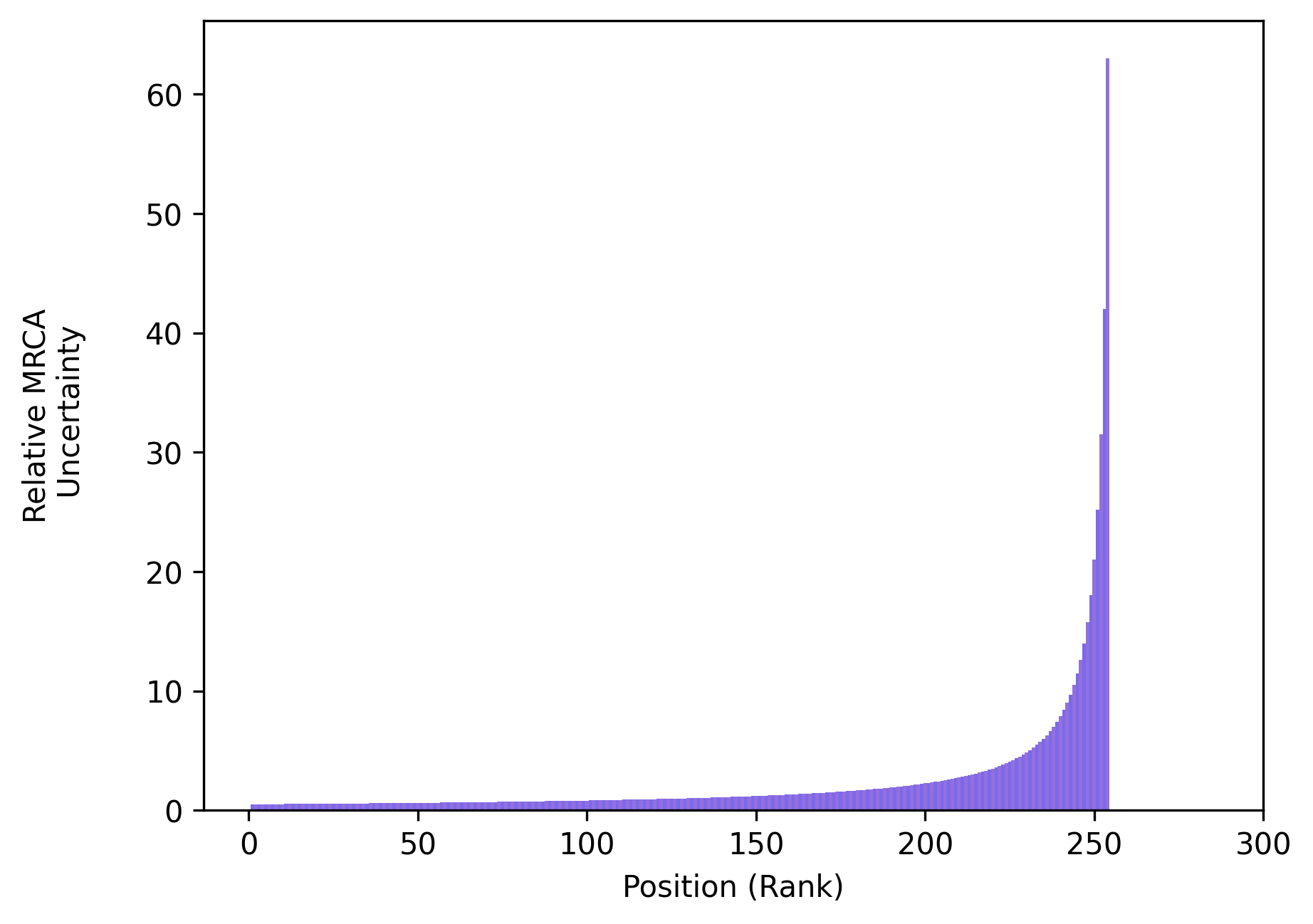
Num Strata Retained	Absolute MRCA Uncertainty by Position	Relative MRCA Uncertainty by Position

Other Algorithms

These stratum retention algorithms are less likely of interest to end users, included in the library primarily for testing and design validation, but are available nonetheless. See API listing for all available algorithms here.

nominal resolution policy
perfect resolution policy
pseudostochastic policy
stochastic policy

Custom Algorithm Design

Custom stratum retention algorithms can easily be substituted for supplied algorithms without performing any modifications to library code. To start, you’ll most likely want to copy an existing algorithm from hstrat/stratum_retention_strategy/stratum_retention_algorithms to use as an API scaffold.

If writing a custom stratum retention algorithm, you will need to consider

Prune sequencing.

When you discard a stratum now, it won’t be available later. If you need a stratum at a particular time point, you must be able to guarantee it hasn’t already been discarded at any prior time point.
Column composition across intermediate generations.

For many use cases, resolution and column size guarantees will need to hold at all generations because the number of generations elapsed at the end of an experiment is not known a priori or the option of continuing the experiment with evolved genomes is desired.
Tractability of computing the deposit generations of retained strata at an arbitrary generation.

If this set of generations can be computed efficiently, then an efficient reverse mapping from column array index to deposition generation can be attained. Such a mapping enables deposition generation to be omitted from strata, potentially yielding a 50%+ space savings (depending on the differentia bit width used).